Note
Click here to download the full example code
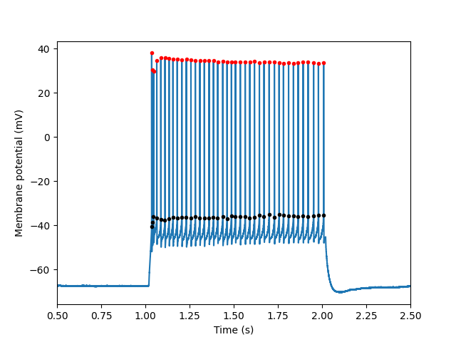
Single sweep detection
Detect spikes for a single sweep
Out:
/home/docs/checkouts/readthedocs.org/user_builds/ipfx/envs/latest/lib/python3.6/site-packages/hdmf/spec/namespace.py:485: UserWarning: Ignoring cached namespace 'hdmf-common' version 1.1.0 because version 1.3.0 is already loaded.
  % (ns['name'], ns['version'], self.__namespaces.get(ns['name'])['version']))
/home/docs/checkouts/readthedocs.org/user_builds/ipfx/envs/latest/lib/python3.6/site-packages/hdmf/spec/namespace.py:485: UserWarning: Ignoring cached namespace 'core' version 2.2.0 because version 2.2.5 is already loaded.
  % (ns['name'], ns['version'], self.__namespaces.get(ns['name'])['version']))
import os
import matplotlib.pyplot as plt
from ipfx.dataset.create import create_ephys_data_set
from ipfx.feature_extractor import SpikeFeatureExtractor

# Download and access the experimental data from DANDI archive per instructions in the documentation
# Example below will use an nwb file provided with the package

nwb_file = os.path.join(
    os.path.dirname(os.getcwd()),
    "data",
    "nwb2_H17.03.008.11.03.05.nwb"
)

# Create data set from the nwb file and choose a sweeep
dataset = create_ephys_data_set(nwb_file=nwb_file)
sweep = dataset.sweep(sweep_number=39)

# Extract information about the spikes
ext = SpikeFeatureExtractor()
results = ext.process(t=sweep.t, v=sweep.v, i=sweep.i)

# Plot the results, showing two features of the detected spikes
plt.plot(sweep.t, sweep.v)
plt.plot(results["peak_t"], results["peak_v"], 'r.')
plt.plot(results["threshold_t"], results["threshold_v"], 'k.')

# Set the plot limits to highlight where spikes are and set axis labels
plt.xlim(0.5, 2.5)
plt.xlabel("Time (s)")
plt.ylabel("Membrane potential (mV)")

plt.show()
Total running time of the script: ( 0 minutes 1.398 seconds)